Filter node
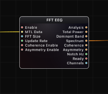
FFT EEG
Real-time multi-channel EEG spectral analysis node. Processes raw brainwave data from a BrainBrick Device Input into clinically relevant frequency band powers, full power spectral density, cross-channel coherence, and hemispheric asymmetry metrics -- all output as structured JSON for visualization, conditional logic, and downstream processing.
Inputs
| Port | Type | Default |
|---|---|---|
| EnableOff stops the analysis and drops the collected samples, so the next start begins from a fresh buffer. | bool | true |
| EEG DataThe multi-channel EEG to analyse: EEG Data from BrainBrick Device Input, or a Signal in µV (EEG Stream Receive, Signal Channels, a filter). An empty or disconnected source simply keeps the last analysis on the outputs. | structure | — |
| FFT SizeSamples per analysis window — bigger means finer frequency detail but a slower, more sluggish reading. Snapped to the nearest power of two within 1024…131072, and further reduced if the incoming buffer cannot hold two windows. | int | 65536 |
| Update RateHow many analyses per second to run. 0 means as often as new data allows; a few per second is plenty for smooth band values and costs far less. | float | 0.0 |
| Coherence EnableTurns on the pairwise coherence output, which measures how synchronised two electrodes are. Off by default because it costs extra work every analysis. | bool | false |
| Asymmetry EnableTurns on the left-versus-right asymmetry output for mirrored electrode pairs. Off by default because it costs extra work every analysis. | bool | false |
Outputs
| Port | Type |
|---|---|
| Analysis | json |
| Total Power | json |
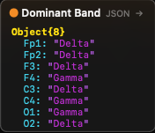
| Dominant Band | json |
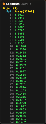
| Spectrum | json |
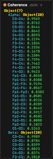
| Coherence | json |
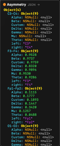
| Asymmetry | json |
| Notch Hz | float |
| Ready | bool |
| Channels | int |
Screenshots
Live Preview
Signal Processing Pipeline
The FFT EEG node implements a complete EEG signal processing chain. Data flows through the following stages:
1. Ingestion (MainActor, ~50 us)
Raw interleaved samples are read from the BrainBrick Device Input's shared MTLBuffer (Metal Unified Memory, zero-copy). The ingestion step:
- De-interleaves the multi-channel data from
[ch0_sample0, ch1_sample0, ch0_sample1, ch1_sample1, ...]into per-channel arrays. - Handles ring buffer wraparound (the MTLBuffer is circular; the read position may wrap to the beginning).
- Tracks the write head position to read only new samples since the last frame.
- Detects gaps (if delta >= maxFrames, the buffer has wrapped completely and data is stale — triggers a full reset).
- Detects buffer changes (device reconnection creates a new MTLBuffer — triggers a full reset).
2. DC Removal (per sample)
A very slow exponential moving average (EMA) tracks the DC baseline of each channel:
- Time constant: tau = 10 seconds at 16 kHz --> -3 dB at 0.016 Hz
- This is well below the lowest EEG band (Delta starts at 0.5 Hz), so no EEG signal is affected
- Purpose: removes large DC offsets from the ADC before they reach the IIR filter, preserving Float32 precision
3. High-Pass Filter (4th-order Butterworth)
A 4th-order Butterworth high-pass filter (two cascaded 2nd-order biquad sections) removes residual sub-Hz drift:
- Default cutoff: 0.1 Hz (configurable in Settings)
- True 4th-order pole placement: Q1 = 0.5412, Q2 = 1.3066
- 80 dB/decade rolloff for effective drift removal
- Implemented using
vDSP_biquad(Apple Accelerate framework) with Double-precision coefficients and Float I/O
4. Notch Filter (powerline removal)
Removes 50 Hz or 60 Hz powerline interference plus harmonics:
- Fundamental — Two cascaded 2nd-order IIR notch filters at the center frequency for >-40 dB attenuation
- 2nd harmonic (100/120 Hz) — Two more cascaded notch sections (optional, enabled by Harmonics setting)
- 3rd harmonic (150/180 Hz) — Two more cascaded notch sections (optional)
- Configurable Q factor (default 30.0) — higher Q = narrower notch = less signal loss near the center frequency
- Adaptive mode — Tracks the actual powerline frequency by detecting the peak in the PSD near the nominal frequency, with EMA smoothing and hysteresis
5. Welch PSD Computation (Actor, ~5 ms, GPU or CPU)
Power spectral density is computed using Welch's averaged periodogram method:
- The internal buffer (3x FFT size per channel) is segmented into overlapping windows
- Default overlap: 50% (configurable) — with 3x buffer, this yields approximately 5 averaged segments
- Each segment is mean-subtracted (robust DC removal independent of HP filter)
- Optional linear detrend removes any remaining linear drift within the segment
- A window function is applied (Hanning default, Hamming, or Blackman available)
- Forward FFT via
vDSP_fft_zrip(CPU) or Metal compute shader (GPU) - Magnitude-squared spectrum is computed and scaled to one-sided PSD density (uV^2/Hz)
- PSD arrays from all segments are averaged to reduce variance
The computation is dispatched to a dedicated FFTEEGProcessor actor. Only one FFT task runs per node at a time (guard prevents overlap). Results are stored in an atomic cache (os_unfair_lock) for zero-cost synchronous reads from the MainActor.
GPU acceleration — When available, the node uses a Metal compute shader (WelchPSDMetalEngine) for the windowing, FFT, and PSD computation stages. The CPU path serves as an automatic fallback. All channels are processed in parallel via DispatchQueue.concurrentPerform.
6. Band Power Extraction
After PSD computation, absolute and relative power are calculated for each frequency band:
- Absolute power = sum of PSD bins within band x frequency resolution (integrated power in uV^2)
- Relative power = band power / total power (fraction, 0 — 1)
- Peak frequency = frequency of the highest PSD bin within the band
- Peak amplitude = PSD value at the peak frequency
- Dominant band = band with the highest absolute power (excluding Custom and Mu)
7. Artifact Detection
If enabled, channels with total power exceeding the artifact threshold (default 500 uV^2) are flagged. Artifact-flagged channels:
- Are marked with
"artifact": truein the Analysis output - Have their asymmetry results reported as null when both channels in a pair are flagged
- Are still included in coherence computation (user may filter downstream)
8. Coherence Computation (optional)
Magnitude-squared coherence (MSC) measures the linear relationship between two channels at each frequency:
Coh_xy(f) = |<S_xy(f)>|^2 / (<S_xx(f)> x <S_yy(f)>)Where <...> denotes averaging over multiple segments. Range: 0 (no relationship) to 1 (perfect linear relationship).
Critical implementation detail: Single-segment coherence is always 1.0 (Cauchy-Schwarz identity). Meaningful coherence requires multi-segment averaging. The node uses shorter 4096-point segments with 50% overlap from the full buffer, yielding approximately 30 segments for robust averaging.
All channel pairs are computed in parallel. The output is grouped by frequency band, with each band containing coherence values for all configured pairs (or all unique pairs if none are configured).
9. Asymmetry Computation (optional)
Hemispheric asymmetry index (AI) quantifies power differences between left and right hemisphere electrodes:
AI(band) = (Power_right - Power_left) / (Power_right + Power_left)Range: -1.0 (left dominant) to +1.0 (right dominant), 0.0 = symmetric.
Computed per band for each configured left/right channel pair. If no pairs are configured, adjacent channels are paired automatically (0-1, 2-3, 4-5, ...).
Frequency Bands
| Band | Default Range | Typical EEG Association |
|---|---|---|
| Delta | 0.5 — 4 Hz | Deep sleep, unconsciousness, brain injury markers |
| Theta | 4 — 8 Hz | Drowsiness, light sleep, meditation, memory encoding |
| Alpha | 8 — 12 Hz | Relaxed wakefulness, eyes closed, occipital dominance |
| Beta | 12 — 30 Hz | Active thinking, focus, anxiety, motor planning |
| Gamma | 30 — 90 Hz | Higher cognitive functions, perception, consciousness |
| Mu | 8 — 13 Hz | Sensorimotor rhythm (overlaps Alpha), suppressed by movement/motor imagery |
| Custom | 0.5 — 100 Hz | User-defined range, configurable in Settings |
All band boundaries are configurable in the node's Settings tab. The Custom band allows monitoring any frequency range of interest.
Settings (Inspector)
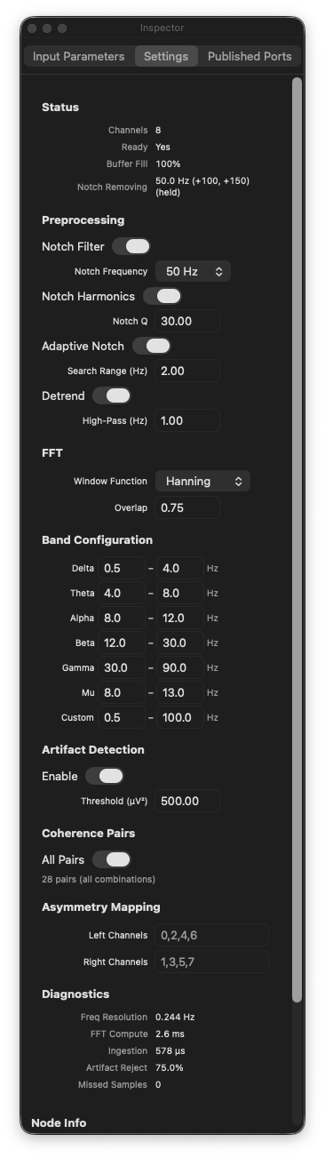
The FFT EEG node has extensive settings accessible through the Inspector panel's Settings tab:
Preprocessing
| Setting | Default | Description |
|---|---|---|
| Notch Filter | On | Enable/disable powerline interference removal. |
| Notch Frequency | 50 Hz | Select 50 Hz (Europe, Asia, Africa) or 60 Hz (Americas, Japan). |
| Harmonics | On | Also filter 2nd and 3rd harmonics (100/120 Hz, 150/180 Hz). |
| Notch Q | 30.0 | Quality factor of the notch filter. Higher = narrower notch. |
| Adaptive Notch | Off | Automatically detect and track the actual powerline frequency. |
| Search Range | 2.0 Hz | How far from the nominal frequency to search in adaptive mode. |
| Detrend | On | Apply linear detrend to each FFT segment before windowing. |
| High-Pass Hz | 0.1 | High-pass filter cutoff frequency. |
FFT
| Setting | Default | Description |
|---|---|---|
| Window Function | Hanning | Window applied to each FFT segment. Options: Hanning (best general-purpose for EEG), Hamming (slightly different sidelobe behavior), Blackman (lowest leakage, wider main lobe). |
Artifact Detection
| Setting | Default | Description |
|---|---|---|
| Artifact Detection | On | Enable automatic artifact flagging per channel. |
| Threshold | 500.0 uV^2 | Total power above this value flags the channel as artifact. |
Band Ranges
Each of the 7 bands (Delta, Theta, Alpha, Beta, Gamma, Mu, Custom) has configurable min/max frequency boundaries in Hz.
Coherence
| Setting | Default | Description |
|---|---|---|
| Coherence Pairs | (empty) | Specify which channel pairs to compute. Format: 0-1,0-2,1-3. Empty = all unique pairs. |
Asymmetry
| Setting | Default | Description |
|---|---|---|
| Left Channels | (empty) | Comma-separated channel indices for the left hemisphere (e.g. 0,2,4). |
| Right Channels | (empty) | Comma-separated channel indices for the right hemisphere (e.g. 1,3,5). Pairs are formed by matching position: left[0]-right[0], left[1]-right[1], etc. |
Output JSON Structures
Analysis Output
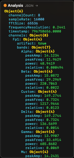
The Analysis port outputs a complete JSON structure with this layout:
{
  "channelCount": 8,
  "sampleRate": 16000,
  "fftSize": 65536,
  "frequencyResolution": 0.244,
  "timestamp": 1711929600.123,
  "channels": {
    "Fp1": {
      "artifact": false,
      "totalPower": 42.5,
      "dominantBand": "Alpha",
      "bands": {
        "Delta": {
          "power": 8.2,
          "relative": 0.193,
          "peakFreq": 2.5,
          "peakAmp": 1.8
        },
        "Theta": {
          "power": 5.1,
          "relative": 0.120,
          "peakFreq": 6.0,
          "peakAmp": 1.2
        },
        "Alpha": {
          "power": 15.8,
          "relative": 0.372,
          "peakFreq": 10.2,
          "peakAmp": 4.5
        },
        "Beta": {
          "power": 7.3,
          "relative": 0.172,
          "peakFreq": 18.5,
          "peakAmp": 0.8
        },
        "Gamma": {
          "power": 3.1,
          "relative": 0.073,
          "peakFreq": 40.0,
          "peakAmp": 0.3
        },
        "Mu": {
          "power": 12.0,
          "relative": 0.282,
          "peakFreq": 10.5,
          "peakAmp": 3.9
        },
        "Custom": {
          "power": 42.5,
          "relative": 1.0,
          "peakFreq": 10.2,
          "peakAmp": 4.5
        }
      }
    },
    "Fp2": { ... },
    "F3": { ... }
  }
}
Channel keys use electrode labels from the BrainBrick Device Input when available, or numeric indices ("0", "1", ...) otherwise. Channels are sorted in anatomical front-to-back order (Fp, F, C, P, T, O) for consistent output regardless of device channel ordering.
Band power fields:
power— Absolute band power in uV^2 (integrated PSD over band range)relative— Fraction of total power (0 — 1)peakFreq— Frequency of the highest PSD bin within the band, in HzpeakAmp— PSD amplitude at the peak frequency, in uV^2/Hz
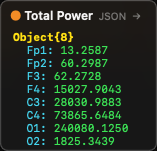
Total Power Output
{
  "Fp1": 42.5,
  "Fp2": 38.7,
  "F3": 51.2,
  "F4": 49.8
}
Per-channel total integrated power in uV^2. Keys in anatomical order.
Dominant Band Output
{
  "Fp1": "Alpha",
  "Fp2": "Alpha",
  "F3": "Beta",
  "F4": "Theta"
}
The name of the frequency band with the highest absolute power per channel (excluding Custom and Mu from the competition).
Spectrum Output
{
  "Fp1": [0.001, 0.002, 0.015, 0.234, ...],
  "Fp2": [0.001, 0.003, 0.012, 0.198, ...],
  "_bandRanges": [
    {"name": "Delta", "min": 0.5, "max": 4.0},
    {"name": "Theta", "min": 4.0, "max": 8.0},
    ...
  ]
}
Each channel maps to an array of PSD values (uV^2/Hz) from bin 0 (DC) to bin N/2 (Nyquist). The frequency of bin i is i x frequencyResolution. The _bandRanges metadata provides the current band boundary configuration for downstream visualization nodes (such as EEG Spectrum).
Coherence Output
{
  "Alpha": {
    "Fp1-Fp2": 0.85,
    "F3-F4": 0.72,
    "C3-C4": 0.91
  },
  "Beta": {
    "Fp1-Fp2": 0.62,
    "F3-F4": 0.55,
    "C3-C4": 0.78
  },
  "Delta": { ... },
  "Theta": { ... },
  "Gamma": { ... },
  "Mu": { ... },
  "Custom": { ... }
}
Grouped by frequency band. Each band contains magnitude-squared coherence values (0 — 1) for each channel pair. Pair keys use electrode labels when available (e.g. "Fp1-Fp2"), or indices ("0-1").
Interpreting coherence:
- 0.0 — No linear relationship between channels at this frequency band
- 0.5 — Moderate coupling
- 1.0 — Perfect linear relationship (identical signals)
- High alpha coherence between homologous electrode pairs (e.g. C3-C4) is a common healthy-brain marker
- Reduced coherence may indicate disconnection or lesion between brain regions
Asymmetry Output
{
  "Fp1-Fp2": {
    "left": "Fp1",
    "right": "Fp2",
    "Delta": -0.05,
    "Theta": 0.12,
    "Alpha": 0.31,
    "Beta": -0.08,
    "Gamma": 0.02,
    "Mu": 0.28,
    "Custom": 0.15
  },
  "F3-F4": { ... }
}
Each pair key maps to an object containing:
left/right— The electrode labels for the pair- Per-band asymmetry index: -1.0 (left dominant) to +1.0 (right dominant), 0.0 = symmetric
nullif both channels in the pair are artifact-flagged
Interpreting asymmetry:
- Frontal alpha asymmetry (F3-F4, F7-F8) is widely studied as a marker of emotional valence and approach/withdrawal motivation
- Positive alpha asymmetry (right > left) is associated with approach motivation and positive affect
- Negative alpha asymmetry (left > right) is associated with withdrawal motivation
- Values near 0 indicate symmetric hemispheric activity
FFT Size and Frequency Resolution
The FFT Size directly determines frequency resolution:
Frequency Resolution = Sample Rate / FFT Size| FFT Size | Freq Resolution at 16 kHz | Freq Resolution at 256 Hz | Buffer Duration at 16 kHz |
|---|---|---|---|
| 1024 | 15.625 Hz | 0.250 Hz | 0.064 s |
| 4096 | 3.906 Hz | 0.0625 Hz | 0.256 s |
| 16384 | 0.977 Hz | 0.0156 Hz | 1.024 s |
| 32768 | 0.488 Hz | -- | 2.048 s |
| 65536 | 0.244 Hz | -- | 4.096 s |
| 131072 | 0.122 Hz | -- | 8.192 s |
For EEG analysis, a frequency resolution of 0.5 Hz or better is typically desired to resolve individual frequency bands. At 16 kHz sample rate, FFT Size 32768 (0.488 Hz resolution) or 65536 (0.244 Hz, the default) are good choices.
Trade-off: Larger FFT sizes give finer frequency resolution but require more samples before the first result (longer startup delay) and more computation time.
Architecture and Performance
Three-Phase Architecture
The node uses a carefully designed three-phase architecture to maintain 120 fps output rendering while performing computationally expensive FFT analysis:
- Ingestion phase (MainActor, ~50 us) — De-interleaves samples from the shared MTLBuffer and applies real-time IIR filters. Runs every frame with new data available.
- FFT computation phase (FFTEEGProcessor actor, ~5 ms) — Dispatched as a fire-and-forget Task. At most one FFT task runs per node at a time (guard prevents overlap). Computes Welch PSD, band powers, coherence, and asymmetry on a dedicated actor with per-channel parallelism.
- Result read phase (MainActor, ~0 us) — Cached FFT results are stored behind an
os_unfair_lockand read synchronously with zero overhead. The output always reflects the most recently completed FFT computation.
Performance Characteristics
| Metric | Typical Value | Notes |
|---|---|---|
| Ingestion per frame | ~50 us | De-interleave + IIR filter, scales with delta samples x channels |
| FFT computation | ~5 ms | Welch PSD via GPU Metal or CPU parallel, 8 channels, 65536 FFT |
| Coherence computation | ~2 ms | 4096-point segments, all pairs, parallel |
| Result cache read | ~0 us | Lock-protected atomic read |
| Internal buffer per channel | 3x FFT size | 196608 samples at default settings |
| Memory per channel | ~768 KB | 3 x 65536 x 4 bytes |
Multiple Instances
Multiple FFT EEG nodes can run simultaneously in the same graph. Each node maintains independent per-node state (ingestion buffers, filter states, FFT cache). This allows analyzing the same device data with different FFT sizes or settings, or analyzing data from different devices.
Practical EEG Analysis Tips
Getting Started
- Add a BrainBrick Device Input node and connect to your EEG device
- Add an FFT EEG node and connect the MTL Data output to its MTL Data input
- Wait for the Ready output to become
true(a few seconds for the buffer to fill) - Connect the Analysis output to a JSON Break node to inspect per-channel results
- Connect the Spectrum output to an EEG Spectrum visualization node
Optimizing for Real-Time BCI
- Set Update Rate to 4 — 10 Hz to balance responsiveness with CPU usage
- Use FFT Size 32768 for faster startup with adequate resolution
- Disable Coherence and Asymmetry unless needed — they add significant computation
- Monitor the inspector's performance diagnostics (ingestion time, FFT time, buffer fill %)
Interpreting Band Powers
- Relative power (0 — 1) is often more useful than absolute power for comparisons across channels or sessions, as it normalizes for overall signal amplitude differences
- Alpha power typically increases when the subject closes their eyes and decreases when they open them (the classic "alpha blocking" effect)
- Beta power increases during active cognitive engagement
- Theta/Alpha ratio is sometimes used as a drowsiness index
- Frontal midline theta (Fz) is associated with sustained attention and working memory
Artifact Management
- Keep the artifact threshold at 500 uV^2 for typical EEG amplitudes
- Sudden spikes in Total Power across all channels often indicate movement artifact
- Single-channel artifacts may indicate a loose electrode
- The artifact flag is per-channel and per-computation — it does not reject data from the buffer, only marks the current epoch
Notch Filter Configuration
- Use 50 Hz in Europe, Asia, and most of the world; 60 Hz in the Americas and parts of Asia (Japan, Taiwan)
- Enable Harmonics to also remove 2nd and 3rd harmonic interference (100/120 Hz, 150/180 Hz)
- The Adaptive Notch mode is useful when the exact powerline frequency varies (e.g. generator power) — it tracks the actual peak and adjusts the notch center frequency with EMA smoothing
- A Q of 30 provides a narrow notch that minimally affects surrounding frequencies. Lower Q values (10 — 20) remove more interference but also attenuate more EEG signal near the notch frequency
Typical Graph Configurations
Basic EEG Analysis
BrainBrick Device Input --> FFT EEG --> JSON Break --> [per-channel band powers]
                                  --> EEG Spectrum --> Canvas
Full Analysis with Visualization
BrainBrick Device Input --> FFT EEG (Coherence On, Asymmetry On)
    Analysis --> JSON Break --> JSON Get (path: "channels.Fp1.bands.Alpha.relative") --> UI Text
    Spectrum --> EEG Spectrum --> Canvas
    Total Power --> JSON Break --> [per-channel power bars]
    Coherence --> JSON Get --> [pair coherence values]
    Asymmetry --> JSON Get --> [hemisphere asymmetry display]
Neurofeedback Loop
BrainBrick Device Input --> FFT EEG
    Analysis --> JSON Get (channels.Cz.bands.Alpha.relative) --> Compare (> 0.3) --> [reward trigger]
                                                              --> Remap (0..0.5 to 0..1) --> Circle 2D (Radius) --> Canvas
Window Functions
| Function | Frequency Resolution | Spectral Leakage | Best For |
|---|---|---|---|
| Hanning | Good | Low | General-purpose EEG analysis (default). Best balance of resolution and leakage. |
| Hamming | Good | Low (slightly different sidelobe pattern) | Similar to Hanning. Does not reach zero at window edges. |
| Blackman | Reduced (wider main lobe) | Lowest | When spectral leakage from strong nearby signals is a concern (e.g. strong powerline near gamma band). |
For most EEG applications, Hanning is the recommended choice.
Understanding the Output Values
This section explains every value returned by the FFT EEG node in plain language, with analogies, typical ranges, and practical examples — written for users who are not deeply familiar with EEG signal processing.
Think of the equalizer in a music player — it shows how loud the bass, mid, and treble frequencies are. The FFT EEG node does the same thing with brain signals, except the frequency bands correspond to different brain states.
Why uV² (Squared) and Not Just uV?
There are two ways to measure an EEG signal:
| Unit | What it measures | Analogy |
|---|---|---|
| uV (microvolts) | Amplitude — how tall the signal wave is | Height of an ocean wave (cm) |
| uV² (microvolts squared) | Power — how much energy is in the signal | Wave energy (height²) |
Simple analogy: Think of ocean waves.
- Amplitude (uV) = wave height, for example 10 cm.
- Power (uV²) = wave energy, which is proportional to height squared: 10² = 100.
A basic physics law: energy is proportional to amplitude². Therefore:
- If the signal amplitude is 5 uV then power is 25 uV²
- If the signal amplitude is 10 uV then power is 100 uV²
- Double the amplitude = four times the power
Why use power (uV²) instead of amplitude (uV)?
- The EEG signal oscillates around zero (+ and − values). If you simply summed amplitudes, positive and negative waves would cancel each other out, giving a result near zero.
- By squaring the amplitudes, all values become positive, and the sum truly reflects the signal's strength.
- This is the standard method in spectral analysis (Welch PSD), used by every EEG system worldwide.
In short: uV = "how tall the wave is", uV² = "how much energy is in the wave". The FFT EEG node works with power (energy), so you will see uV² everywhere.
Total Power — Typical Values
| State | Typical value | Description |
|---|---|---|
| Relaxed person, eyes closed | 5–30 uV² | Normal EEG |
| Active thinking | 3–15 uV² | Reduced alpha, increased beta |
| Muscle artifact | 100–1000+ uV² | Abnormally high — artifact |
| Electrode fell off | 0.001 or less | Near zero — no signal |
| Sleep state | 20–80 uV² | Increased delta/theta |
Range:
- Min: ~0.0 (no signal or very weak signal)
- Max: theoretically unlimited, but in practice >500 uV² is almost always an artifact
- Typical operating range: 1–50 uV²
Practical example: To control an object's size in a visualization based on overall signal strength, use totalPower with a Remap node:
- Input:
totalPower(range 1–50) - Output: object size (range 0.1–1.0)
Dominant Band — Brain State Mapping
| Value | Meaning | Typical state |
|---|---|---|
"Delta" | Slow waves dominate (0.5–4 Hz) | Deep sleep, unconsciousness |
"Theta" | Theta waves dominate (4–8 Hz) | Drowsiness, meditation, imagination |
"Alpha" | Alpha waves dominate (8–12 Hz) | Relaxation with eyes closed |
"Beta" | Beta waves dominate (12–30 Hz) | Active thinking, concentration |
"Gamma" | Gamma waves dominate (30–90 Hz) | Intense cognitive processing |
"None" | Cannot determine | Not enough data |
Note: Mu and Custom bands are excluded from dominant band determination because Mu overlaps with Alpha, and Custom is user-defined.
Practical example: Change the background color based on the dominant band:
"Alpha"→ green background (relaxation)"Beta"→ blue background (concentration)"Theta"→ purple background (meditation)
Band Power — Typical Ranges
| Band | Frequency range | Typical power (uV²) at rest | What increases it |
|---|---|---|---|
| Delta | 0.5–4 Hz | 1–10 | Sleep, fatigue, brain injury |
| Theta | 4–8 Hz | 0.5–5 | Meditation, imagination, memory processes |
| Alpha | 8–12 Hz | 2–15 | Eyes closed, relaxation |
| Beta | 12–30 Hz | 1–8 | Active thinking, stress, concentration |
| Gamma | 30–90 Hz | 0.1–3 | High-level cognitive processing |
| Mu | 8–13 Hz | 1–10 | Motor rest state (disappears during movement) |
| Custom | 0.5–100 Hz | varies | User-defined range |
Practical example: Alpha power is the most commonly used parameter in neurofeedback:
- Subject closes eyes → Alpha power increases from 3 to 12 uV²
- Subject opens eyes → Alpha power drops to 2 uV²
- Goal: teach the subject to increase Alpha power with eyes open (relaxation training)
Relative Power — Proportions
What it is: The proportion of a band's power relative to the total power. Answers the question: "What percentage of the total signal does this band make up?"
Unit: dimensionless ratio, range 0.0 to 1.0
Formula: relative = power / totalPower
| Value | Meaning | Example |
|---|---|---|
| 0.0 | This band is not present in the signal | No alpha waves |
| 0.15 | 15% of the total signal is this band | Normal theta proportion |
| 0.40 | 40% of the total signal is this band | Very strong alpha (relaxation) |
| 0.60 | 60% of the total signal is this band | Dominant band |
| 1.0 | 100% — the entire signal is this band | Practically impossible |
Important: The sum of all bands' relative values is approximately 1.0 (exactly 1.0 when using only the standard non-overlapping bands).Why relative matters: Absolute power varies between people (some naturally have a stronger signal than others). Relative power lets you compare proportions regardless of signal strength.
Peak Frequency — Individual Variability
What it is: The frequency with the highest power amplitude within the band. Answers: "Where exactly within the band is the strongest signal?"
| Band | peakFreq range | Typical value | What affects it |
|---|---|---|---|
| Delta | 0.5–4.0 Hz | 1.5–3.0 Hz | Sleep depth |
| Theta | 4.0–8.0 Hz | 5.0–7.0 Hz | Meditation intensity |
| Alpha | 8.0–12.0 Hz | 9.5–11.0 Hz | Individual Alpha Frequency (IAF) |
| Beta | 12.0–30.0 Hz | 14.0–22.0 Hz | Type of thinking |
| Gamma | 30.0–90.0 Hz | 35.0–50.0 Hz | Cognitive load |
| Mu | 8.0–13.0 Hz | 9.0–11.0 Hz | Motor readiness |
Practical example — Individual Alpha Frequency (IAF):
Each person has their own alpha peak. One person may be at 9.5 Hz, another at 11.2 Hz. IAF is an important biomarker:
- IAF > 10.5 Hz → Faster cognitive processing
- IAF < 9.0 Hz → Possible cognitive slowing
- IAF shifting left (decreasing) → Fatigue, aging
- Use
Alpha.peakFreqto track IAF in real time
Peak Amplitude — Sharp vs Diffuse Peaks
What it is: The PSD value (power spectral density) at the frequency bin where the band's maximum occurs. Shows how pronounced the peak is.
Unit: uV²/Hz
| peakAmp value | Meaning |
|---|---|
| < 0.1 | Very weak peak — band is barely present |
| 0.5–2.0 | Normal EEG peak |
| 2.0–10.0 | Strong peak (e.g., strong alpha during relaxation) |
| > 10.0 | Very strong — check for artifacts |
Difference between power and peakAmp:
power= the band's total power (width x height)peakAmp= only the tallest point within the band
Think of a mountain range:
power= the total volume of the entire rangepeakAmp= the highest summit- You can have a tall summit (
peakAmp) but a narrow range (smallpower) - Or a low but very wide range (large
power, smallpeakAmp)
Practical example: Use peakAmp to determine whether the alpha peak is "sharp" (a distinct rhythm) or "flat" (a diffuse signal):
Alpha.peakAmp > 3.0andAlpha.relative > 0.3→ Clear alpha rhythm (good relaxation state)Alpha.peakAmp < 0.5butAlpha.power > 2.0→ Diffuse signal in the alpha band (no distinct rhythm)
Coherence — Interpreting Synchronization
| Value | Meaning |
|---|---|
| 0.0 | Completely unsynchronized — channels operate independently |
| 0.3 | Weak coherence |
| 0.5 | Moderate coherence |
| 0.7 | High coherence — channels are functionally connected |
| 1.0 | Perfect synchronization (practically impossible in biological signals) |
Practical example: Alpha coherence between frontal channels (F3–F4) can indicate:
- High (>0.6): Frontal symmetry — emotional balance
- Low (<0.3): Frontal asymmetry — possible risk of depression
Asymmetry — Hemispheric Balance
| Value | Meaning |
|---|---|
| -1.0 | Complete left-side dominance |
| -0.3 | Moderate left dominance |
| 0.0 | Symmetric signal |
| +0.3 | Moderate right dominance |
| +1.0 | Complete right-side dominance |
Practical example — Frontal Alpha Asymmetry (FAA):
- FAA > 0 (right > left alpha) → Positive emotions, approach motivation
- FAA < 0 (left > right alpha) → Negative emotions, withdrawal motivation
- Used in depression and emotional state research
Note: If both channels in a pair are flagged as artifacts, band values are set to null. If only one channel is an artifact, the AI is still calculated normally. If the combined power of both channels is very small (< 1e-10 uV²), AI = 0 (symmetric).
Quick Reference — Typical Value Scenarios
Scenario: Person sitting quietly with eyes closed
| Parameter | Fp1 (Frontal) | O1 (Occipital) |
|---|---|---|
| totalPower | 15 uV² | 25 uV² |
| dominantBand | "Alpha" | "Alpha" |
| Alpha.power | 4.5 uV² | 12.0 uV² |
| Alpha.relative | 0.30 | 0.48 |
| Alpha.peakFreq | 10.25 Hz | 10.25 Hz |
| Alpha.peakAmp | 1.5 uV²/Hz | 4.8 uV²/Hz |
| Beta.power | 3.2 uV² | 1.8 uV² |
| Beta.relative | 0.21 | 0.07 |
| artifact | false | false |
Note: Alpha is stronger in occipital channels (O1, O2) than in frontal channels (Fp1, Fp2) — this is normal.
Scenario: Person actively solving a math problem
| Parameter | Fp1 (Frontal) | O1 (Occipital) |
|---|---|---|
| totalPower | 10 uV² | 12 uV² |
| dominantBand | "Beta" | "Beta" |
| Alpha.power | 1.2 uV² | 2.5 uV² |
| Alpha.relative | 0.12 | 0.21 |
| Beta.power | 4.8 uV² | 3.9 uV² |
| Beta.relative | 0.48 | 0.33 |
| Beta.peakFreq | 18.5 Hz | 16.1 Hz |
Note: Beta is higher in frontal channels (thinking), Alpha has decreased (eyes open, active state).
Useful Formulas for Neurofeedback and BCI
Theta/Beta Ratio (Attention Indicator)
TBR = Theta.power / Beta.power| Ratio | Meaning |
|---|---|
| > 3.0 | Risk of attention deficit |
| 1.5–2.5 | Normal resting state |
| < 1.0 | High concentration |
Note on relative values: Therelativevalue itself is always between 0.0 and 1.0 (it is a proportion). But if you divide one relative by another, the result can exceed 1.0. Example: ifTheta.relative = 0.30andBeta.relative = 0.10, then ratio = 0.30 / 0.10 = 3.0. This means there is 3x more energy in the Theta band than in the Beta band.
Alpha Ratio (Relaxation Indicator)
Alpha_ratio = Alpha.relative| Value | Meaning |
|---|---|
| > 0.35 | Deep relaxation |
| 0.15–0.35 | Normal calm |
| < 0.10 | Active/stressed state |
Engagement Index
EI = Beta.power / (Alpha.power + Theta.power)| Value | Meaning |
|---|---|
| > 1.0 | High engagement |
| 0.5–1.0 | Moderate engagement |
| < 0.5 | Low engagement, drowsiness |
Spectrum Data — How to Use the Raw PSD Array
Each channel in the Spectrum output contains a float array with halfN elements (e.g., 32768 elements with FFT Size = 65536). Each element is the power spectral density at a specific frequency.
The array index corresponds to a frequency:
frequency_Hz = index x frequencyResolutionExample (16000 Hz sample rate, 65536 FFT size, frequencyResolution = 0.244 Hz):
| Array index | Frequency (Hz) | Typical PSD value | What is happening there |
|---|---|---|---|
| 0 | 0 Hz (DC) | ~0 | Empty (DC removed) |
| 1 | 0.24 Hz | 0.005 | Very low frequency |
| 20 | 4.88 Hz | 0.15 | Theta range |
| 41 | 10.01 Hz | 2.30 | Alpha peak |
| 80 | 19.53 Hz | 0.08 | Beta range |
| 200 | 48.83 Hz | 0.001 | Higher frequencies, very little power |
| 32767 | 7999.8 Hz | ~0.0 | Near Nyquist frequency |
PSD Value Ranges
| PSD value (uV²/Hz) | Meaning |
|---|---|
| < 0.01 | Very low power — background noise |
| 0.01–0.5 | Normal EEG activity |
| 0.5–5.0 | Pronounced band peak (e.g., alpha rhythm) |
| 5.0–50.0 | Very strong signal — check for artifacts |
| > 50.0 | Almost certainly an artifact |
Practical Uses for Raw Spectrum Data
- Spectrogram: Store PSD arrays over time to build a 2D color map where X = time, Y = frequency, color = power. This is a "brain activity heat map".
- Individual frequency analysis: To know the exact power at 10.0 Hz:
index = 10.0 / 0.244 = 41, thenpower_at_10Hz = Spectrum["Fp1"][41]. - Custom band definition: Use the Spectrum data to compute your own band sum:
my_band_power = sum(Spectrum[i]) x 0.244whereicovers your desired frequency range. - EEG Spectrum visualization: Connect the Spectrum output directly to an EEG Spectrum node, which renders it as a frequency graph.
Technical Parameters Summary
| Parameter | Value | Note |
|---|---|---|
| Sample Rate | 16000 Hz | From BrainBrick device |
| FFT Size | 65536 (default) | Range: 1024–131072 |
| Frequency Resolution | ~0.244 Hz | = 16000/65536 |
| Nyquist Frequency | 8000 Hz | = 16000/2 |
| Welch Segments | ~3–24 | Depends on buffer size |
| Overlap | 50% (default) | Adjustable 0–90% |
| Window Function | Hanning (default) | Options: Hanning, Hamming, Blackman |
| Computation Engine | Metal GPU | ~2 ms on Apple Silicon |
| Update Rate | 0 Hz (default) | Every frame; increase to limit |
A ready-made example project for this node is built into Grafit Pro: select the node in the library and open or drag the example from its description panel.
Open FFT EEG in the interactive catalog →
FFT EEG is one of 381 nodes in Grafit Pro.
Free download. Every feature for 7 days, no card. Then €99.99 once — or keep playing your projects as a Player.